[Explained] How to Hide or Unhide Columns in Excel

Do you want to hide or unhide columns in Excel but don’t know how to? If yes, you have stumbled upon the right webpage.

Microsoft Excel is among the most powerful data management tools. Known for its user-friendly interface and comprehensive features, its ability to handle massive amounts of data efficiently is incomparable.

But despite that, handling large datasets in Excel could become overwhelming. The excessive data often results in cluttering the UI, causing inefficiency. And that’s when Excel’s ability to hide and unhide columns comes into play.

Here, I have covered a detailed guide covering the advantages of hiding columns in Excel, different ways to do so, and more.

So, without any further ado, let’s get started –

Use Cases for Hiding/Unhiding Columns

Hiding and unhiding columns in Excel can offer several benefits, contributing to a more efficient and organized data management process.

Here are some of the practical use cases –

✅ Organize large data – Working on large data can be tiresome and overwhelming and could make the spreadsheet look cluttered. In such a situation, you could use the hide function to declutter the spreadsheet and organize data. This would help you with easier navigation, simplified data analysis, space management, and more.

✅ Hide critical data – While presenting your spreadsheet data to others, you could use the hide columns function to hide sensitive data such as sales figures, account or login details, personal details, etc.

✅ Create custom views – Custom view is a feature in Excel that allows you to create specific display and print settings for a worksheet. You can create multiple custom views tailored for specific purposes by hiding or unhiding columns in Excel.

So, these are some of Excel’s most common use cases of hiding or unhiding columns.

How To Hide Columns in Excel

So far, I have covered the most common use cases and the importance of hiding and unhiding columns in Excel.

And now, let’s discuss a few simple methods to hide columns in Excel –

#1. Using Mouse

This is arguably one of Excel’s simplest and best methods to hide columns.

To hide columns in Excel using your mouse, you need to follow these simple steps –

cryptoshitcompra.com/wp-content/uploads/2023/11/Explained-How-to-Hide-or-Unhide-Columns-in-Excel.png", "imageCurrentSrc": "", "targetWidth": "717", "targetHeight": "369", "scaleAttr": "", "dialogLabel": "Enlarged image" } } }» data-wp-interactive=»» class=»wp-block-image size-full is-resized wp-lightbox-container»>

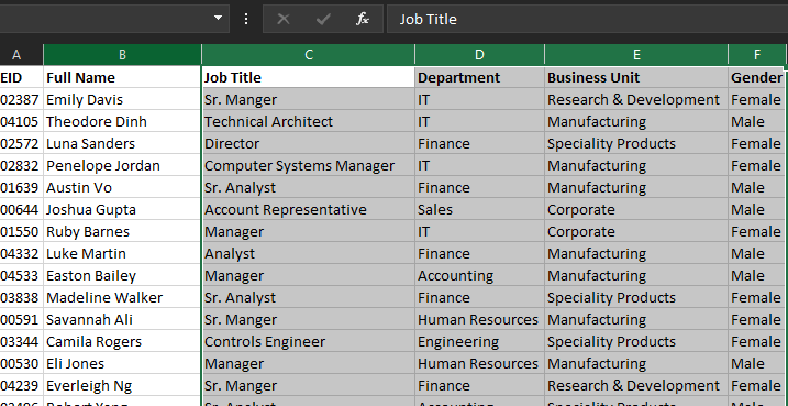
• Right-click on any of the selected columns to open the Context menu.
• Select the Hide option in the context menu.

png", "imageCurrentSrc": "", "targetWidth": "843", "targetHeight": "523", "scaleAttr": "", "dialogLabel": "Enlarged image" } } }» data-wp-interactive=»» class=»wp-block-image size-full is-resized wp-lightbox-container»>

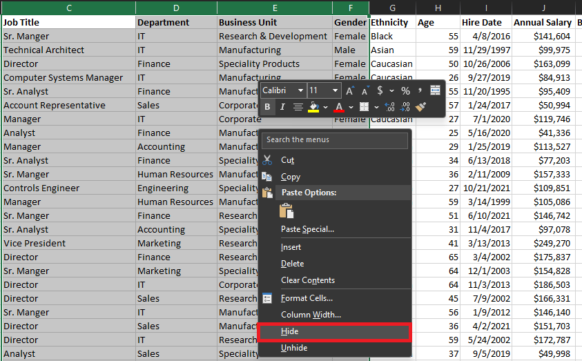
That’s it. This is how you can easily hide columns in Excel just using your mouse.

#2. Using Shortcut

The mouse method to hide columns in Excel is great, but there is a fancy way to do the same. You can hide columns in Excel using the Excel keyboard shortcut. The only limitation here is that you will have to use your mouse if you want to hide multiple non-adjacent columns.

Here is how to hide columns in Excel using the Excel keyboard shortcut –

• First of all, open the Excel sheet that contains the columns you want to hide.
• Select the columns you want to hide. To select adjacent columns, follow these steps –
  • Go to the first column you want to select.
  • Press the Shift + Left or Right Arrow keys to select the columns you want to hide.
  • After that, press CTRL + Spacebar to ensure the columns are selected instead of rows.

If the columns are non-adjacent, press the CTRL key and then choose the columns using your mouse.

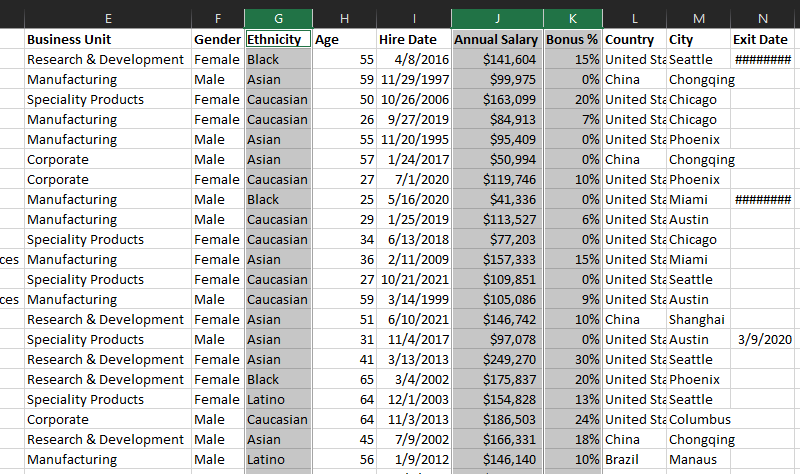
•  Once the columns are selected, press the CTRL + 0 key to hide all the selected columns.

Doing so will instantly hide all the selected columns in Excel.

#3. Using Format Function

The Format function in Excel is a very versatile tool designed to format a wide range of data. It is mainly used for conditional formatting but can also be used to customize the appearance of numbers, dates, text strings, special characters, etc.

The Format function can also help you hide and unhide Excel columns and rows. Here is how you can do that –

• First of all, open the Excel file.
• Select all the columns you want to hide.

• Make sure you are in the Home tab of the Excel ribbon.
• Select the Format option listed under the Cells menu. This will open a drop-down context menu.
• Hover over the Hide & Unhide option listed under Visibility and then select the Hide Columns option.

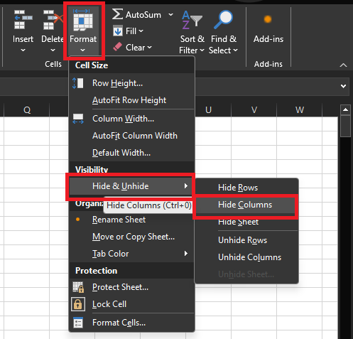
That’s it. This is how you can easily hide columns in Excel using the Format function.

#4. Using VBA

VBA, which stands for Visual Basic for Application, is a programming language that can help you automate tasks, create custom rules, and overall extend the functionality of Excel. You can use VBA to create a simple macro to hide columns in Excel.

Here is a step-by-step guide to do that –

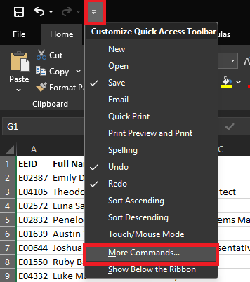
• First of all, open the Excel sheet and check whether the Developer option is visible in the ribbon. If the option isn’t there, follow the steps from two to five. Otherwise, you can skip these steps.
• Now, click the drop-down arrow icon in the Quick Access Toolbar. This will open a context menu.
• Select the More Commands… option.

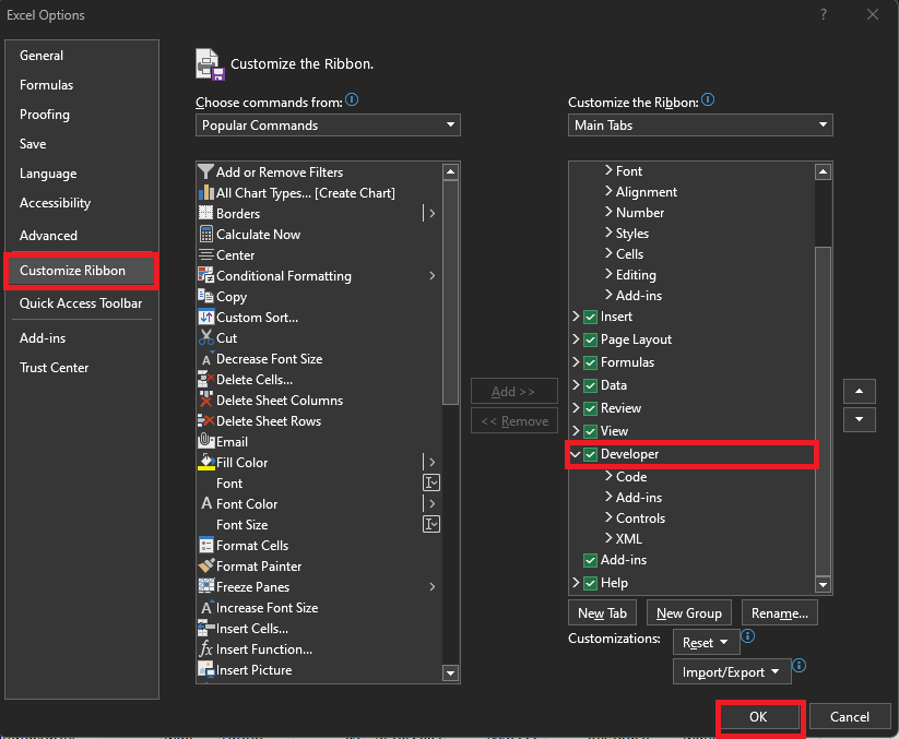
• Excel Options pop-up menu will appear. Here, select the Customize Ribbon option from the left sidebar.
• Mark the checkbox associated with the Developer option checked and click the OK button.

• Now, select the Developer tab in the ribbon and click on the Visual Basic function. This will launch the VBA editor.

• Click on the Insert menu in the toolbar and then select the Module option. This will launch a module for your spreadsheet.

• Here, you need to write the code to hide the column. The thing here is that you need to write custom code to hide specific columns, and I cannot teach you everything here. But I have shared the basic code.
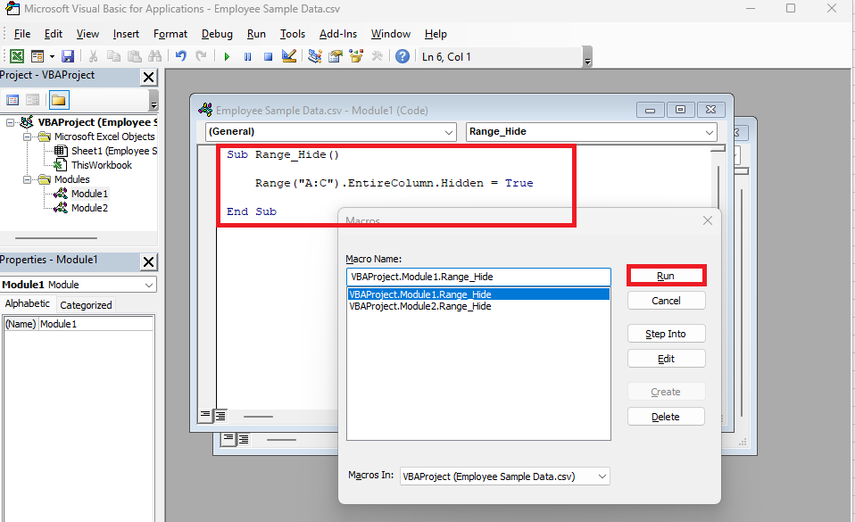
• To hide multiple adjacent or single columns in Excel, you need to write the following code –

Sub Range_Hide()

    Range("A:C").EntireColumn.Hidden = True

End Sub

Here, we are asking to hide columns ranging from A to C (“A:C”). This means all the columns between A and C, including A and C, will be hidden after running this code.

You can also hide a single column with the same code. Just replace (“A:C”) with (“A:A”) or any other column of your choice and run the code.

• After writing the code, press F5 to run the macro. This will open a pop-up where you need to select the Run option.

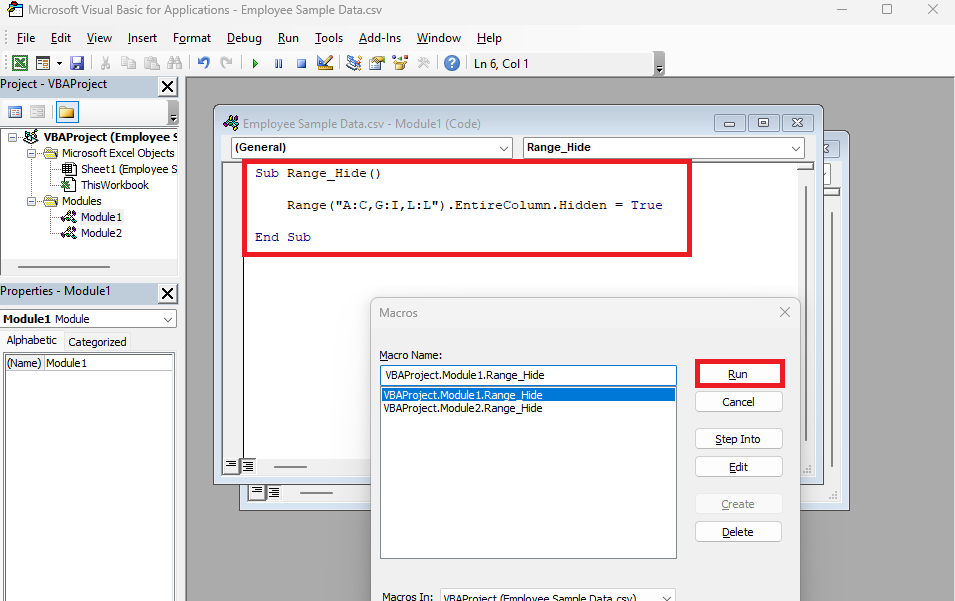
• Alternatively, if you want to hide specific columns, you can write the following code –

Sub Range_Hide()

    Range("A:C,G:I,L:L").EntireColumn.Hidden = True

End Sub

Here, we declare to hide columns ranging from A to C, G to I, and L. You can replace these columns in your code to hide the columns of your choice.

• After that, press F5 and select the Run option to execute the code.

That’s it. This is how you can hide columns in Excel using VBA.

#5. Using Custom View

The Custom View function is best when you want to view or present specific information on a heavily crowded spreadsheet.

Follow these steps to hide columns in Excel using the Custom View function –

• First of all, open your Excel sheet.
• Click on the View tab and select the Custom Views function.

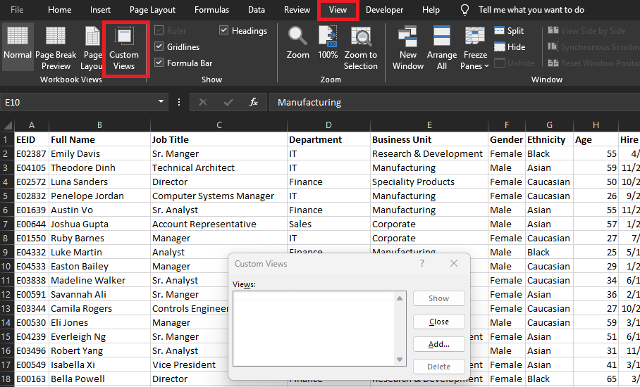
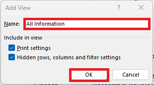
• Click on the Add button, give this Custom View a name, and click the OK button. This way, we have created a sheet that contains all the information.

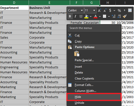
• Now, select the columns you want to hide.
• Right-click on the selected columns and select the Hide option in the context menu.

• After that, click on the Custom Views option again in the View tab.
• Select the Add option, give this Custom View a name, and then click on the OK button.

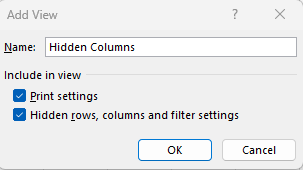
That’s it. You can now easily toggle between both custom views by following these simple steps:

• Go to the View tab in the ribbon.
• Select the Custom View option.
• A pop-up window will appear. Here, you can see all the created Custom Views.
• Select the Custom View you want to open and click on the Show button.

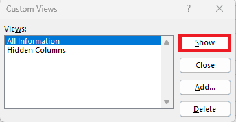
This is how you can easily hide columns using the Custom View function and toggle between available custom views.

#6. Using Group Function

Next, we have the method to hide columns in Excel using the Group function. In this method, we basically group adjacent columns, and then we can expand or hide them as per requirements.

Here is how you can use the Group function –

• First of all, open the Excel sheet.
• Select all the adjacent columns that you want to hide.
• After that, go to the Data tab in the ribbon.
• Select the Group function listed under Outline settings in the toolbar.
• Select the Group option.

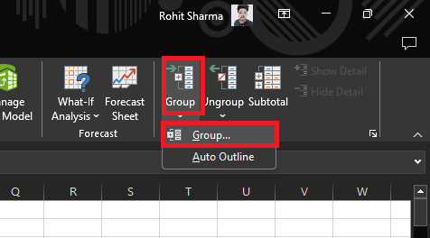
• After grouping the columns, you can see the Plus (+) or Minus (-) icon at the top of the hidden columns.
• Select the Minus (-) to hide selected columns.

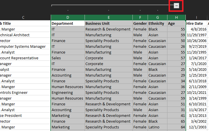
That’s it. This is how you can hide columns in Excel using the Group function.

How to Unhide Columns in Excel

So far, we have covered a few different methods to hide columns in Excel, and now it’s time to cover a few methods to unhide columns.

#1. Using Go To

To unhide columns in Excel using this method, you need to follow these simple steps –

• First, open the Excel sheet.
• Identify the hidden columns.
• Select the left and the right columns of the hidden columns.
• Right-click on the selected column to open the context menu.
• Select the Unhide option.

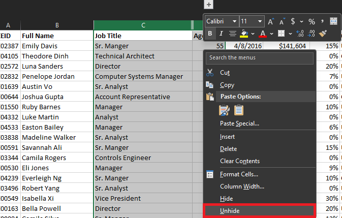
That’s it. This is how you can easily unhide columns in Excel using your mouse only.

#2. Using Expand Feature

If you have hidden the Excel columns using the Group method shared above, you can easily unhide them by following these simple steps –

• Open the Excel sheet.
• First, we need to identify the hidden columns. The hidden columns will most likely have a Plus (+) icon on top of it.
• After you find the Plus (+) icon, click on it.

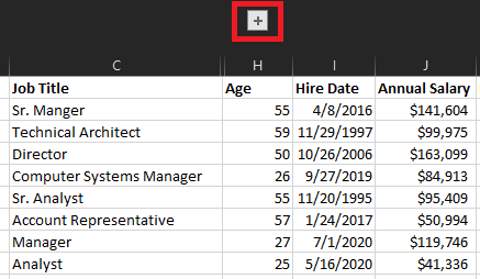
That’s it. Doing so will unhide the grouped columns.

If you have multiple columns hidden in groups, you need to expand all those groups to unhide all the hidden columns.

#3. Using Custom View

This method only works if you have hidden the columns using the Custom View method.

Follow these simple steps to unhide columns using the Custom View method –

• First, open the Excel sheet.
• Go to the View tab and select the Custom Views option under the Workbook Views function.
• Select the Custom View with no hidden columns in the Custom Views pop-up.
• Click on the Show button.

That’s it. This will present you with a Custom View that has no hidden columns.

#4. Using Keyboard Shortcut

Another way to unhide columns in Excel is by using the Excel keyboard shortcut. This method is quite similar to the Go To method. But the only difference is that we will use the keyboard shortcut here.

Follow these simple steps to unhide columns in Excel using the keyboard shortcut –

• Open the Excel sheet.
• Select the adjacent columns of the hidden columns.
• Now press the CTRL + Shift + 0 keys together.

Doing so will unhide the selected hidden columns.

Closing Comments

There you have it – a detailed article covering information about how to hide and unhide columns in Excel.

When working on spreadsheets containing sensitive or massive data, the hiding/unhiding column feature appears as a lifesaver. By using these features, you cannot only protect sensitive data but also declutter the sheet and make it easier to work on.

Next, check out the online Excel courses for beginner to advanced levels.