NLP Simplified: Part II – Types of Vectorization Techniques

In this article, we will discuss vectorization – an NLP technique, and understand its significance with a comprehensive guide on different types of vectorization.

We have discussed the fundamental concepts of NLP preprocessing and text cleaning. We looked at the basics of NLP, its various applications, and techniques like tokenization, normalization, standardization, and text cleaning.

Before we discuss Vectorization, let’s revise what tokenization is and how it differs from vectorization.

What is Tokenization?

Tokenization is the process of breaking down sentences into smaller units called tokens. Token helps computers to understand and work with text easily.

EX. ‘This article is good’

Tokens- [‘This’, ‘article’, ‘is’, ‘good’.]

What is Vectorization?

As we know, machine learning models and algorithms understand numerical data. Vectorization is a process of converting textual or categorical data into numerical vectors. By converting data into numerical data, you can train your model more accurately.

Why Do We Need Vectorization?

❇️ Tokenization and vectorization have different importance in natural language processing (NPL). Tokenization breaks sentences into small tokens. Vectorization converts it into a numerical format so the computer/ML model can understand it.

❇️ Vectorization is not only useful for converting it to numerical form but also useful in capturing semantic meaning.

❇️ Vectorization can reduce the dimensionality of the data and make it more efficient. This could be very useful while working on a large dataset.

❇️ Many machine learning algorithms require numerical input, such as neural networks, so that vectorization can help us.

There are different types of vectorization techniques, which we will understand through this article.

Bag of Words

If you have a bunch of documents or sentences and you want to analyze them, a Bag of Words simplifies this process by treating the document as a bag that is filled with words.

The bag of words approach can be useful in text classification, sentiment analysis, and document retrieval.

Suppose, you are working on lots of text. A bag of words will help you to represent text data by creating a vocabulary of unique words in our text data. After creating vocabulary, It will encode each word as a vector based on the frequency (how often each word appears in that text) of these words.

These vectors consist of non-negative numbers (0,1,2…..) that represent the number of frequencies in that document.

The bag of words involves three steps:

Step 1: Tokenization

It will break documents into tokens.

Ex – (Sentence: “I love Pizza and I love Burgers”)

Step 2: Unique word separation/vocabulary creation

Create a list of all the unique words that appear in your sentences.

[“I”, “love”, “Pizza”, “and”, “Burgers”]

Step 3: Counting word occurrence/ vector creation

This step will count how many times each word is repeated from the vocabulary and store it in a sparse matrix. In the sparse matrix, each row in a sentence vector whose length (the columns of the matrix) is equal to the size of the vocabulary.

Import CountVectorizer

We are going to import CountVectorizer to train our Bag of words model

from sklearn.feature_extraction.text import CountVectorizer

Create Vectorizer

In this step, we are going to create our model using CountVectorizer and train it using our sample text document.

# Sample text documents
documents = [
    "This is the first document.",
    "This document is the second document.",
    "And this is the third one.",
    "Is this the first document?",
]

# Create a CountVectorizer 
cv = CountVectorizer()

# Fit and Transform
X = cv.fit_transform(documents)

Convert to a dense array

In this step, we will convert our representations into dense array. Also, we will get feature names or words.

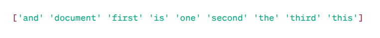
# Get the feature names/words
feature_names = vectorizer.get_feature_names_out()

# Convert to dense array
X_dense = X.toarray()

Let’s print the Document term matrix and feature words

# Print the DTM and feature names
print("Document-Term Matrix (DTM):")
print(X_dense)
print("\nFeature Names:")
print(feature_names)

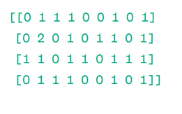
Document – Term Matrix (DTM):

Feature Names:

As you can see, the vectors are consist of non-negative numbers (0,1,2……) which represents frequency of words in document.

We have four sample text documents, and we have identified nine unique words from these documents. We stored these unique words in our vocabulary by assigning them ‘Feature Names.’

Then, our Bag of Words model checks if the first unique word is present in our first document. If it is present, it assigns a value of 1 otherwise, it assigns 0.

If the word appears multiple times (e.g., 2 times), it assigns a value accordingly.

For example, in the second document, the word ‘document’ repeats twice, so its value in the matrix will be 2.

If we want a single word as a feature in the vocabulary key – Unigram representation.

n – grams = Unigrams, bigrams…….etc.

There are many libraries like scikit-learn to implement bag of words: Keras, Gensim, and others. This is simple and can be useful in different cases.

But, Bag of words is faster but it has some limitations.

1. It assigns the same weight to every word, regardless of its importance. In many cases, some words are more important than others.
2. BoW simply counts the frequency of a word or how many times a word appears in a document. This can lead to a bias toward common words like “the”, “and”, “is” etc., which may not carry much meaning.
3. Longer documents may have more word counts and can create larger vectors. This can make it challenging to compare. It can create a sparse matrix, which can’t be good for performing complex NLP projects.

To solve this problem we can choose better approaches, one of them is TF-IDF. Let’s, Understand in detail.

TF-IDF

TF-IDF, or Term Frequency – Inverse Document Frequency, is a numerical representation to determine the importance of words in the document.

Why do we need TF-IDF over Bag of Words?

A bag of words treats all words equally and is just concerned with the frequency of unique words in sentences. TF- IDF gives importance to words in a document by considering both frequency and uniqueness.

Words that get repeated too often don’t overpower less frequent and more important words.

TF: Term Frequency measures how important a word is in a single sentence.

IDF: Inverse document frequency measures how important a word is in the entire collection of documents.

IDF is reciprocal of DF. The reason behind this is the more common the word is across all documents, the lesser its importance in the current document.

Final TF-IDF Score: TF-IDF = TF * IDF

It is a way to find out which words are common within a single document and unique across all documents. These words can be useful in finding the main theme of the document.

For example,

Doc1 = “I love Machine learning”

Doc2 = “I love Geekflare”

We have to find the TF-IDF matrix for our documents.

First, we will create a vocabulary of unique words.

Vocabulary = [“I,” “love,” “machine,” “learning,” “Geekflare”]

So, we have 5 five words. Let’s find TF and IDF for these words.

Now, Let’s calculate the final score of TF-IDF:

• For “I”: TF-IDF for Doc1: 0.25 * 0 = 0 and TF-IDF for Doc2: 0.33 * 0 = 0
• For “love”: TF-IDF for Doc1: 0.25 * 0 = 0 and TF-IDF for Doc2: 0.33 * 0 = 0
• For “Machine”: TF-IDF for Doc1: 0.25 * 0.69 ≈ 0.17 and TF-IDF for Doc2: 0 * 0.69 = 0
• For “Learning”: TF-IDF for Doc1: 0.25 * 0.69 ≈ 0.17 and TF-IDF for Doc2: 0 * 0.69 = 0
• For “Geekflare”: TF-IDF for Doc1: 0 * 0.69 = 0 and TF-IDF for Doc2: 0.33 * 0.69 ≈ 0.23

TF-IDF matrix looks like this:

        I     love   machine   learning   Geekflare
Doc1    0.0   0.0    0.17      0.17       0.0
Doc2    0.0   0.0    0.0       0.0        0.23

Values in a TF-IDF matrix tell you how important each term is within each document. High values indicate that a term is important in a particular document, while low values suggest that the term is less important or common in that context.

TF-IDF is mostly used in text classification, building chatbot information retrieval, and text summarization.

Import TfidfVectorizer

Let’s , import TfidfVectorizer from sklearn

from sklearn.feature_extraction.text import TfidfVectorizer

Create Vectorizer

As you wan see, we will create our Tf Idf model using TfidfVectorizer.

# Sample text documents
text = [
    "This is the first document.",
    "This document is the second document.",
    "And this is the third one.",
    "Is this the first document?",
]

# Create a TfidfVectorizer 
cv = TfidfVectorizer()

Create TF-IDF Matrix

Let’s, train our model by providing text. After that, we will convert the representative matrix to dense array.

# Fit and transform to create the TF-IDF matrix
X = cv.fit_transform(text)

# Get the feature names/words
feature_names = vectorizer.get_feature_names_out()

# Convert the TF-IDF matrix to a dense array for easier manipulation (optional)
X_dense = X.toarray()

Print the TF-IDF Matrix and Feature Words

# Print the TF-IDF matrix and feature words
print("TF-IDF Matrix:")
print(X_dense)
print("\nFeature Names:")
print(feature_names)

TF-IDF Matrix:

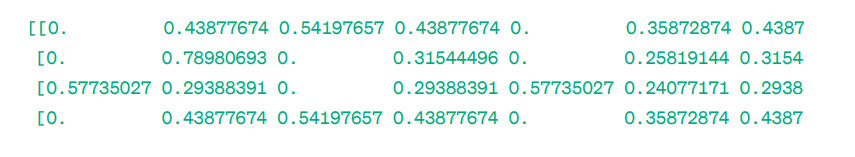
As you can see, these decimal point integers indicate the importance of words in specific documents.

Also, you can combine words in groups of 2,3,4, and so on using n-grams.

There are other parameters that we can include: min_df, max_feature, subliner_tf, etc.

Until now, we have explored basic frequency-based techniques.

But, TF-IDF cannot provide semantic meaning and contextual understanding of text.

Let’s understand more advanced techniques that have changed the world of word embedding and which is better for semantic meaning and contextual understanding.

Word2Vec

Word2vec is a popular word embedding ( type of word vector and useful to capture semantic and syntactic similarity) technique in NLP. This was developed by Tomas Mikolov and his team at Google in 2013. Word2vec represents words as continuous vectors in a multi-dimensional space.

Word2vec aims to represent words in a way that captures their semantic meaning. Word vectors generated by word2vec are positioned in a continuous vector space.

Ex – ‘Cat’ and ‘Dog’ vectors would be closer than vectors of ‘cat’ and ‘girl’.

Two model architectures can be used by word2vec to create word embedding.

CBOW: Continous bag of words or CBOW tries to predict a word by averaging the meaning of nearby words. It takes a fixed number or window of words around the target word, then converts it into numerical form (Embedding), then averages all, and uses that average to predict the target word with the neural network.

Ex- Predict target: ‘Fox’

Sentence words: ‘The’, ‘quick’, ‘brown’, ‘jumps’, ‘over’, ‘the’

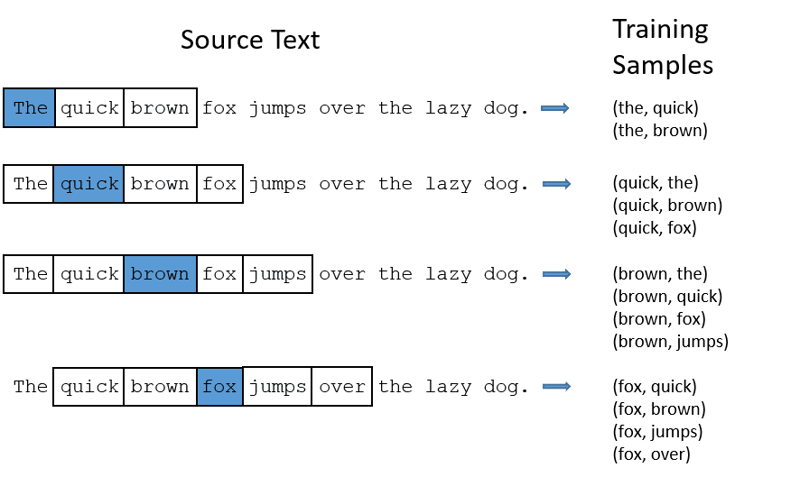
• CBOW takes fixed size window (number) of words like 2 (2 to the left and 2 to the right)
• Convert to word embedding.
• CBOW averages the word embedding.
• CBOW averages the word embedding to the context words.
• Averaged vector tries to predict a target word using a neural network.

Now, Let’s understand how skip-gram is different from CBOW.

Skip-gram: It is a word embedding model, but it works differently. Instead of predicting the target word, skip-gram predicts the context words given target words.

Skip-grams is better at capturing the semantic relationships between words.

Ex- ‘King – Men + Women = Queen’

If you want to work with Word2Vec, you have two choices: either you can train your own model or use a pre-trained model. We will be going through a pre-trained model.

Import gensim

You can install gensim using pip install:

pip install gensim

Tokenize the sentence using word_tokenize:

FIrst, we will convert sentences to lower. After that, we will tokenize our sentences using word_tokenize.

# Import necessary libraries
from gensim.models import Word2Vec
from nltk.tokenize import word_tokenize

# Sample sentences
sentences = [
    "I love thor",
    "Hulk is an important member of Avengers",
    "Ironman helps Spiderman",
    "Spiderman is one of the popular members of Avengers",
]

# Tokenize the sentences
tokenized_sentences = [word_tokenize(sentence.lower()) for sentence in sentences]

Let’s train our model:

We will train our model by providing tokenized sentences. We are using 5 window for this training model, you can adapt as per your requirement.

# Train a Word2Vec model
model = Word2Vec(sentences=tokenized_sentences, vector_size=100, window=5, min_count=1, sg=0)

# Find similar words
similar_words = model.wv.most_similar("avengers")

# Print similar words
print("Similar words to 'avengers':")

for word, score in similar_words:
    print(f"{word}: {score}")

Similar words to ‘avengers’:

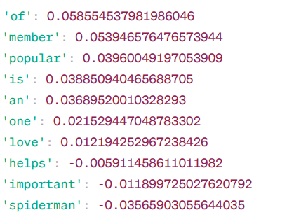
These are some of the words that are similar to “avengers” based on the Word2Vec model, along with their similarity scores.

The model calculates a similarity score (mostly cosine similarity) between the word vectors of “avengers” and other words in its vocabulary. The similarity score indicates how closely related two words are in the vector space.

Ex –

Here, word ‘helps‘ with cosine similarity -0.005911458611011982 with word ‘avengers‘. The negative value suggests that they might dissimilar with each other.

Cosine similarity values range from -1 to 1, where:

• 1 indicates that the two vectors are identical and have positive similarity.
• Values close to 1 indicate high positive similarity.
• Values close to 0 indicate that the vectors are not strongly related.
• Values close to -1 indicate high dissimilarity.
• -1 indicates that the two vectors are totally opposed and have a perfect negative similarity.

Visit this link if you want a better understanding of word2vec models and a visual representation of how they operate. It’s a really cool tool for seeing CBOW and skip-gram in action.

Similar to Word2Vec, we have GloVe. GloVe can produce embeddings that require less memory compared to Word2Vec. Let’s, understand more about GloVe.

GloVe

Global vectors for word representation (GloVe) is a technique like word2vec. It is used to represent words as vectors in continuous space. The concept behind GloVe is the same as Word2Vec’s: it produces contextual word embeddings while taking into consideration Word2Vec’s superior performance.

Why do we need GloVe?

Word2vec is a window-based method, and it uses nearby words to understand words. This means the semantic meaning of the target word is only affected by its surrounding words in sentences, which is an inefficient use of statistics.

Whereas GloVe captures both global and local statistics to come with word embedding.

When to use GloVe?

Use GloVe when you want word embedding that captures broader semantic relationships and global word association.

GloVe is better than other models on named entity recognition tasks, word analogy, and word similarity.

First, We need to Install Gensim:

pip install gensim

Step 1: We are going to install important libraries

# Import the required libraries

import numpy as np
import matplotlib.pyplot as plt
from sklearn.manifold import TSNE
import gensim.downloader as api  

Step 2: Import Glove model

import gensim.downloader as api
glove_model = api.load('glove-wiki-gigaword-300')

Step 3: Retrieve vector word representation for the word ‘cute’

glove_model["cute"]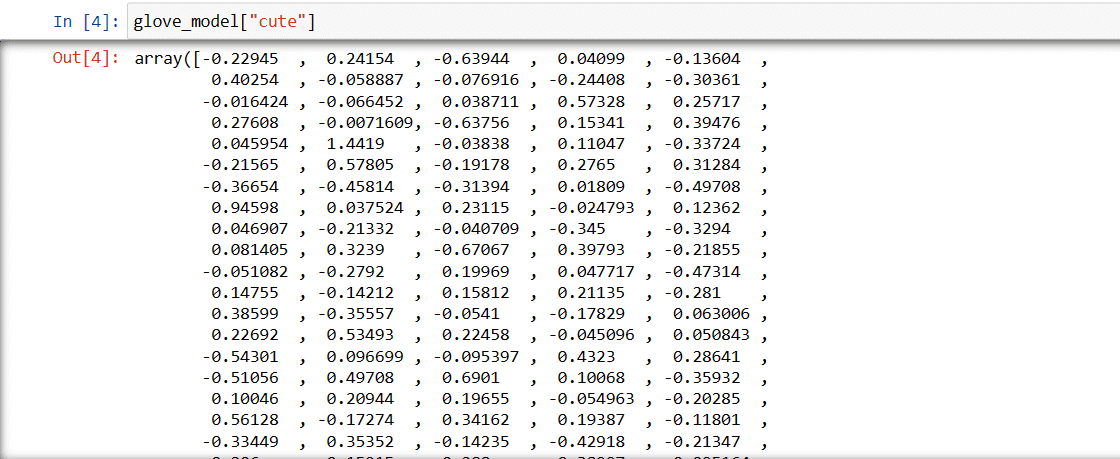

These values capture the word’s meaning and relationships with other words. Positive values indicate positive associations with certain concepts, while negative values indicate negative associations with other concepts.

In a GloVe model, each dimension in the word vector represents a certain aspect of the word’s meaning or context.

The negative and positive values in these dimensions contribute to how “cute” is semantically related to other words in the model’s vocabulary.

Values can be different for different models. Let’s find some simlilar words to word ‘boy’

Top 10 Similar words which model thinks are most similar to the word ‘boy’

# find similar word
glove_model.most_similar("boy")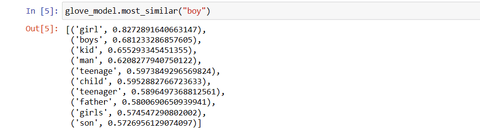

As you can see, most similar word to ‘boy’ is ‘girl’.

Now, we will try to find How accurately the model will get semantic meaning from the provided words.

glove_model.most_similar(positive=['boy', 'queen'], negative=['girl'], topn=1)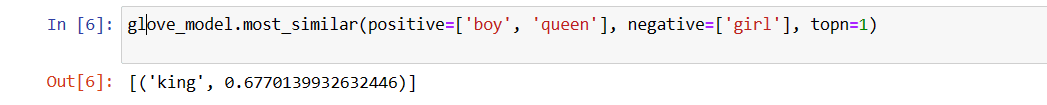

Our model is able to find perfect relationship between words.

Define vocab list:

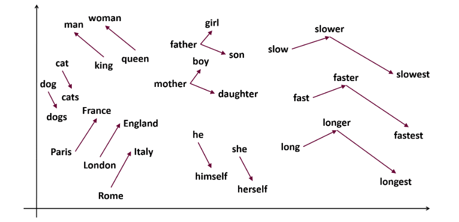
Now, Let’s try to understand semantic meaning or relationship between words using a plot. Define the list of words you want to visualize.

# Define the list of words you want to visualize
vocab = ["boy", "girl", "man", "woman", "king", "queen", "banana", "apple", "mango", "cow", "coconut", "orange", "cat", "dog"]

Create embedding matrix:

Let’s, write code for creating embedding matrix.

# Your code for creating the embedding matrix
EMBEDDING_DIM = glove_model.vectors.shape[1]
word_index = {word: index for index, word in enumerate(vocab)}
num_words = len(vocab)
embedding_matrix = np.zeros((num_words, EMBEDDING_DIM))

for word, i in word_index.items():
    embedding_vector = glove_model[word]
    if embedding_vector is not None:
        embedding_matrix[i] = embedding_vector

Define a function for t-SNE visualization:

From this code, we will define function for our visualization plot.

def tsne_plot(embedding_matrix, words):
    tsne_model = TSNE(perplexity=3, n_components=2, init='pca', random_state=42)
    coordinates = tsne_model.fit_transform(embedding_matrix)

    x, y = coordinates[:, 0], coordinates[:, 1]

    plt.figure(figsize=(14, 8))
    for i, word in enumerate(words):
        plt.scatter(x[i], y[i])
        plt.annotate(word,
                     xy=(x[i], y[i]),
                     xytext=(2, 2),
                     textcoords='offset points',
                     ha='right',
                     va='bottom')
    plt.show()

Let’s see how our Plot looks:

# Call the tsne_plot function with your embedding matrix and list of words
tsne_plot(embedding_matrix, vocab)

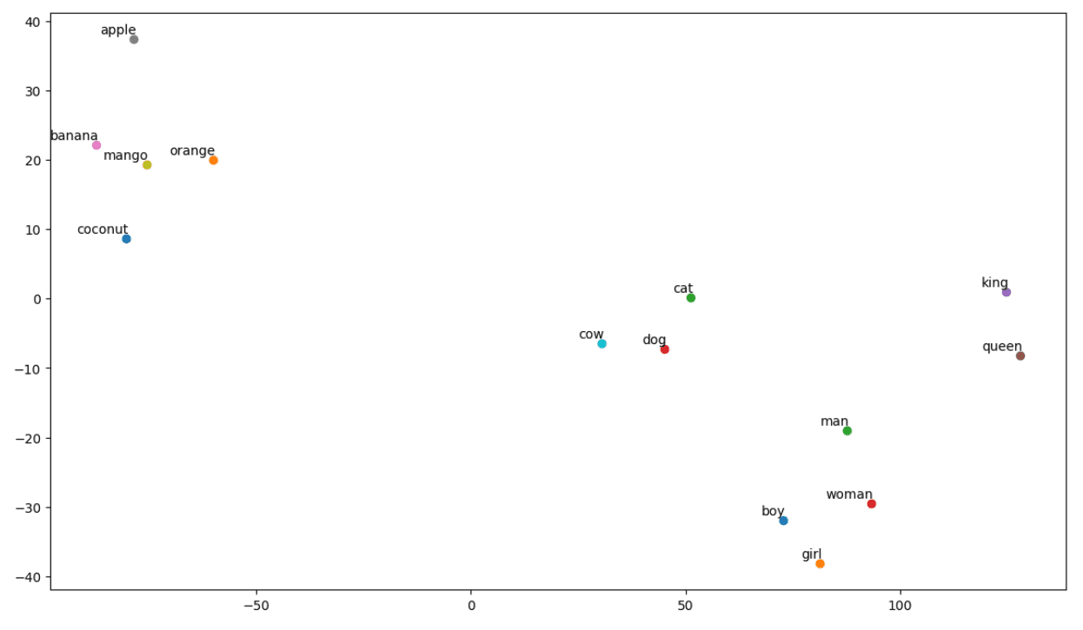
So, as we can see, there are words like ‘banana’, ‘mango’, ‘orange’, ‘coconut’, and ‘apple’ on the left side of our plot. Whereas ‘cow’, ‘dog’, and ‘cat’ are similar to each other because they are animals.

So, our model can find semantic meaning and relationships between words also!

By just changing the vocab or creating your model from scratch, you can experiment with different words.

You can use this embedding matrix however you like. It can be applied to word similarity tasks alone or fed into a neural network’s embedding layer.

GloVe trains on a co-occurrence matrix to derive semantical meaning. It is predicated on the idea that word-word co-occurrences are an essential piece of knowledge and that their use is an effective way to use statistics to produce word embeddings. This is how GloVe accomplishes adding “global statistics” to the final product.

And that’s GloVe; Another popular method for vectorization is FastText. Let’s discuss more about it.

FastText

FastText is an open-source library introduced by Facebook’s AI Research team for text classification and sentiment analysis. FastText provides tools for training word embedding, which are dense vector represent words. This is useful for capturing the semantic meaning of the document. FastText supports both multi-label and multi-class classification.

Why FastText?

FastText is better than other models because of its capability to generalize to unknown words, which had been missing in other methods. FastText provides pre-trained word vectors for different languages, which could be useful in various tasks where we need previous knowledge about words and their meaning.

How does it work?

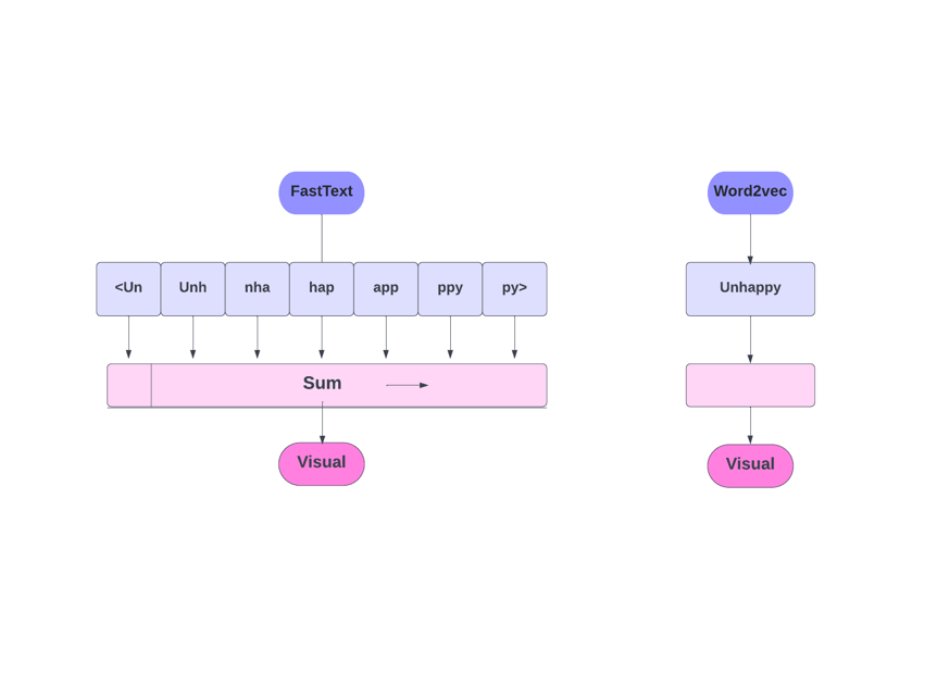
As we discussed, other models, like Word2Vec and GloVe, use words for word embedding. But, the building block of FastText is letters instead of words. Which means they use letters for word embedding.

Using characters instead of words has another advantage. Less data is needed for training. As a word becomes its context, resulting in more information can be extracted from the text.

Word Embedding obtained via FastText is a combination of lower-level embeddings.

Now, let’s look at how FastText utilizes sub-word information.

Let’s say we have the word ‘reading’. For this word, character n-grams of length 3-6 would be generated as follows:

• The beginning and end are indicated by angular brackets.

• Hashing is used because there could be a large number of n-grams; instead of learning an embedding for each distinct n-gram, we learn total B embeddings, where B stands for the bucket size. The 2 million bucket size was used in the original paper.

• Each character n-gram, such as “eadi”, is mapped to an integer between 1 and B using this hashing function, and that index has the corresponding embedding.

• By averaging these constituent n-gram embeddings, the full word embedding is then obtained.

• Even if this hashing approach results in collisions, it helps handle the vocabulary size to a great extent.

• The network used in FastText is similar to Word2Vec. Just like there, we can train the FastText in two modes – CBOW and skip-gram. Thus, we don’t need to repeat that part here again.

You can train your own model, or you can use a pre-trained model. We are going to use a pre-trained model.

First, you need to install FastText.

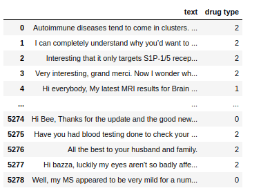
pip install fasttext

We will use a dataset that consists of conversational text regarding a few drugs, and we have to classify those texts into 3 types. Like with the kind of drugs with which they’re associated.

Now, to train a FastText model on any dataset, we need to prepare the input data in a certain format, which is:

__label__<label value&gt;<space&gt;<associated datapoint>

Let’s do this for our dataset, too.

all_texts = train['text'].tolist()
all_labels = train['drug type'].tolist()
prep_datapoints=[]

for i in range(len(all_texts)):
    sample = '__label__'+ str(all_labels[i]) + ' '+ all_texts[i]
    prep_datapoints.append(sample)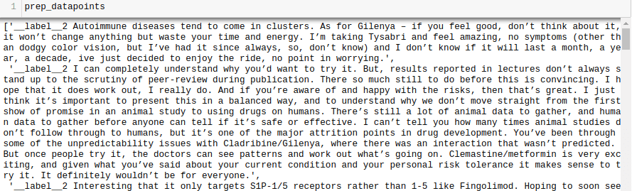

We omitted a lot of preprocessing in this step. Otherwise, our article will be too large. In real-world problems, it’s best to do preprocessing to make data fit for modeling.

Now, write prepared data points to a .txt file.

with open('train_fasttext.txt','w') as f:
    for datapoint in prep_datapoints:
        f.write(datapoint)
        f.write('n')
    f.close()

Let’s train our model.

model = fasttext.train_supervised('train_fasttext.txt')

We will get Predictions from our model.

cryptoshitcompra.com/wp-content/uploads/2023/09/1694739637_457_NLP-Simplified-Part-II-Types-of-Vectorization-Techniques.png«/>

The model predicts the label and assigns a confidence score to it.

Like with any other model, the performance of this one is dependent on a variety of variables, but if you want to get a quick idea of what the expected accuracy is, FastText might be a great option.

Conclusion

In conclusion, text vectorization methods like Bag of Words (BoW), TF-IDF, Word2Vec, GloVe, and FastText provide a variety of capabilities for NLP tasks.

While Word2Vec captures word semantics and is adaptable for a variety of NLP tasks, BoW and TF-IDF are simple and suitable for text classification and recommendation.

For applications like sentiment analysis, GloVe offers pre-trained embeddings, and FastText does well at subword-level analysis, making it useful for structurally affluent languages and entity recognition.

The choice of technique depends on the task, data, and resources. We will discuss the complexities of NLP more deeply as this series progresses. Happy learning!

Next, check out the best NLP courses to learn Natural Language Processing.